Pricing and Adverse Selection
Overview
So far, we’ve focused on health insurance from more of an individual perspective:
- things health insurance does for individuals
- ways to improve health insurance choice or the matching between plans and individuals
But if we want people to have health insurance, and if we care about using a market to allocate health insurance, then we need to take a broader perspective
Estimating Welfare in Insurance Markets Using Variation in Prices
(see Einav, Finkelstein, and Cullen (2010) for details)
Motivation
- Adverse selection is a central concern in health insurance markets
- But very little empirical work in this space (until 2010 or so)
This presumably reflects not a lack of interest in this important topic, but rather the considerable challenges posed by empirical welfare analysis in markets with hidden information.
Basic Model
- Unique feature of adverse selection: demand affects firm costs
- Complicates welfare analysis because we need to know demand curve (how demand varies with price) but also how price changes affect costs
Setup
- Two available contracts: high coverage (\(H\)) and low coverage (\(L\)), with relative price of \(H\) given by \(p\)
- Consumer characteristics \(\zeta\) from distribution \(G(\zeta)\)
- Utility denoted by \(\nu^{H}(\zeta_{i}, p)\) and \(\nu^{L}(\zeta_{i})\) for plan \(H\) and \(L\), respectively
- \(\nu^{H}(\zeta_{i}, p)\) decreasing in \(p\), with \(\nu^{H}(\zeta_{i}, p=0)>\nu^{L}(\zeta_{i})\)
- Costs to insurer given by \(c(\zeta_{i})\)
Demand
- Individual \(i\) choose health insurance if \(\nu^{H}(\zeta_{i}, p)>\nu^{L}(\zeta_{i})\)
- Denote highest price at which individual \(i\) chooses \(H\) as \(\pi(\zeta_{i}) \equiv \max \{p: \nu^{H}(\zeta_{i}, p)>\nu^{L}(\zeta_{i})\}\)
- Aggregate demand, \(D(p) = \int 1(\pi(\zeta) \geq p) dG(\zeta) = Pr(\pi(\zeta) \geq p)\)
Supply
- Bertrand competition with many risk-neutral insurers
- Focus on case of perfect competition as benchmark, so that inefficiency derives from selection and not other factors
- Costs to insurer given by \(c(\zeta_{i})\)
- Average costs are then, \(AC(p) = \frac{1}{D(p)} \int c(\zeta) 1(\pi(\zeta) \geq p) dG(\zeta) = E(c(\zeta) | \pi(\zeta) \geq p)\)
- Marginal costs, \(MC(p) = E(c(\zeta) | \pi(\zeta) = p)\)
- Equilibrium, \(p^{*} = \min \{p : p=AC(p) \}\)
Welfare
Measure welfare using certainty equivalent: amount that would make consumer indifferent between obtaining outcome for sure versus obtaining outcome with uncertainty, denoted \(e^{H}(\zeta_{i})\) and \(e^{L}(\zeta_{i})\), so that WTP for health insurance is reflected by \(\e^{H}(\zeta_{i}) - e^{L}(\zeta_{i})\)
- \(CS = \int \left[ (e^{H}(\zeta) - p)1(\pi(\zeta) \geq p) + e^{L}(\zeta) 1(\pi(\zeta) < p) \right] d G(\zeta)\)
- \(PS = \int \left[ (p - c(\eta)) 1(\pi(\zeta) \geq p) \right] d G(\zeta)\)
- \(TS = CS + PS = \int \left[ (e^{H}(\zeta) - c(\eta)) 1(\pi(\zeta) \geq p) + e^{L}(\zeta) 1(\pi(\zeta) < p) \right] d G(\zeta)\)
- Socially efficient to purchase health insurance only if \(\pi(\eta_{i}) \geq c(\eta_{i})\)
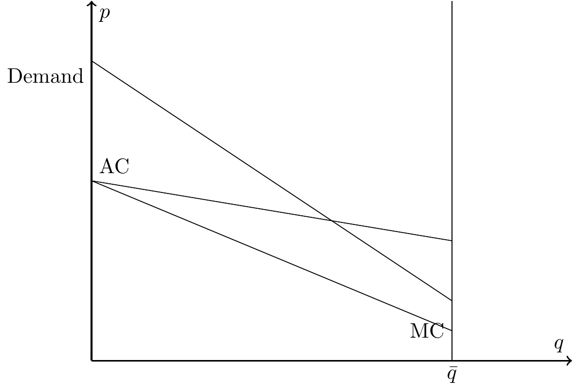
Textbook Adverse Selection
- \(D>MC\) because willingness to pay is expected costs plus risk premium
- Relationship between demand and AC reflects problems due to adverse selection
Main points
- Key assumptions:
- Simplifying assumption that insurers earn 0 profit (at least approximately)
- Individuals select plans based on health needs (which is private information)
- Common price to all enrollees of a given plan (community rating)
- Possible outcomes:
- Full insurance (Demand always above AC)
- Partial unravelling (Demand intersects with AC somewhere)
- Full unravelling (Demand always below AC)
- Limitations
- Only applies to existing contracts
- Cannot speak to entry or exit decisions
Incorporating data
- Goal is to estimate demand curve, \(D(p)\), and average costs, \(AC(p)\)
- \(MC(P)\) derives from product of \(D(p)\) and \(AC(p)\)
- Need data on:
- prices and quantities
- expected costs, such as claims or medical spending
- exogenous shifters in prices
Possible sources of variation
- State regulations introduce variation across people and over time
- Tax policies such as health insurance subisides
- Field experiments and “idiosyncrasies of firm pricing behavior”
- Shifts in administrative costs of handling claims
- Common demand instruments such as plausibly exogenous changes in market conditions
Empirical application
- Health insurance for Alcoa employees in 2004
- “High” versus “low” coverage PPO plans
- Exogenous variation:
- 7 different pricing menus for same coverage
- Focus on relative difference, \(p= p_{H} - p_{L}\)
- Price menus determined by president of business unit
- 40 units in company
“As a result of this business structure, employees doing the same job in the same location may face different prices for their health insurance benefits due to their business unit affiliation.”
- Denote medical expenditures by \(m_{i}\)
- Denote incremental costs by \(c_{i}=c(m_{i}; H) - c(m_{i}; L)\)
- \(c(m_{i}; H)\) is observed
- \(c(m_{i}; L)\) computed based on terms of contract \(L\)
Baseline equations: \[\begin{align*} D_{i} & = \alpha + \beta p_{i} + \epsilon_{i} \\ c_{i} & = \gamma + \delta p_{i} + u_{i} \end{align*}\]
From those: \[MC = \frac{1}{\beta} \frac{ \partial D_{i} c_{i}}{\partial p} = \frac{1}{\beta} (\alpha \delta + \gamma \beta + 2\beta \delta p)\]
Find intersection points and compare to equilibrium points (\(AC(p) = D(p)\)) and efficient points (\(MC(p) = D(p)\))
Pricing and Welfare in Health Plan Choice
(see Bundorf, Levin, and Mahoney (2012) for details)
Motivation
- Prices often not reflective of costs of coverage
- Insurers have incentive to attract specific types of enrollees
- Enrollees have incentive to select specific types of plans
Research question: What are the welfare effects of these forms of selection?
Setup
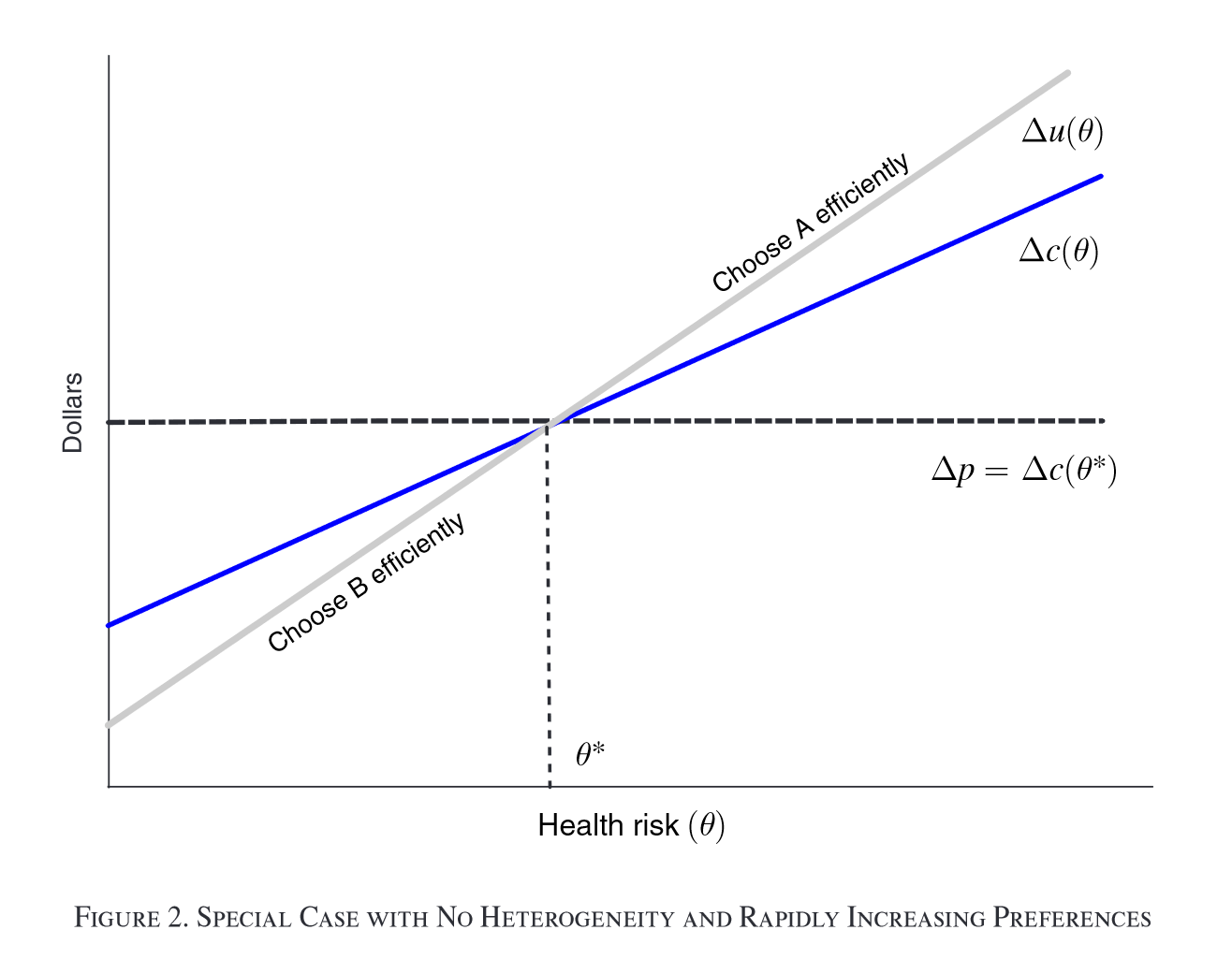
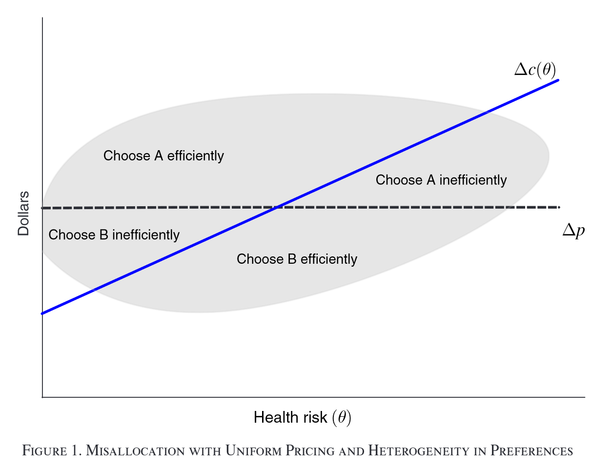
- “Standard” setup with 2 plans
- Assumes WTP $u $ perfectly correlated with health risk \(\theta\)
- Assumes WTP increasing in \(\theta\) faster than costs (i.e., slope of demand curve steeper than slope of AC curve)
Relaxing assumptions yields potential inefficient plan allocation
Data
- “Private firm that helps small and mid-sized employers manage health benefits”
- 11 employers in one metropolitan area in “western United States” from 2004-2005
- Data on 6,603 enrollees (3,683 employees), claims, plan selection, etc.
Model: Demand
Household utility: \[u_{hj} = \alpha_{1} x_{j} + \alpha_{2} x_{h} + \psi (r_{h} + \mu_{h} ; \alpha_{3}) - p_{j} + \sigma_{\varepsilon} \varepsilon_{hj}\]
- \(x_{j}\): plan characteristics
- \(x_{h}\): household characteristics
- \(r_{h}\): health risk score (based on observable demographics)
- \(\mu_{h}\): unobserved health status
- Household \(h\) selects plan \(j\), \(q_{hj} =1\), if \(u_{hj} \geq u_{hk} \forall k \in J_{h}\)
- Standard logit model for plan choice: \[Pr(q_{hj}=1 | x_{h}, \mu_{j}) = \frac{ \exp(v_{hj}) }{ \sum_{k} \exp(v_{hk}) },\]
for \(v_{hj} = u_{hj} - \sigma_{\varepsilon} \varepsilon_{hj}\)
Model: Costs
Costs assumed: \[c_{ij} = a_{j} + b_{j}(r_{i} + \mu_{i} -1) + \eta_{ij}\]
- \(a_{j}\): baseline cost for standard enrollee
- \(b_{j}\): marginal cost of insuring a higher/lower risk enrollee
- Costs for firm-year \(f\) and insurer \(k\) are sum of all relevant \(c_{ij}\)
Model: Other things
- Plan bids: markup over expected costs
- Employer contribution: employers pass on share of lowest-cost plan plus fraction of incremental cost for high-cost plans
Identification and estimation
- Need variation in prices separate from unobserved household tastes or private health risks \(\mu\)
- Instrument for actual plan contribution using predicted contribution
- Estimate using method of simulated moments (simulation comes from draws of \(\mu\) from normal distribution with mean 0 and variance \(\sigma^{2}\):
- Consumer choice: \(E[q_{hj} - Pr(q_{hj}=1 | x_{h}, \mu_{j})|z_{h}, \mu_{h}] = 0\), with instruments \(z_{h}\)
- Plan costs: \(E[C_{kf} - \hat{C}_{kf}|x_{kf}, \mu_{kf}] = 0\)
- Plan bids: \(E[B_{if} - \hat{B}_{if}|x_{f}] = 0\)
Results
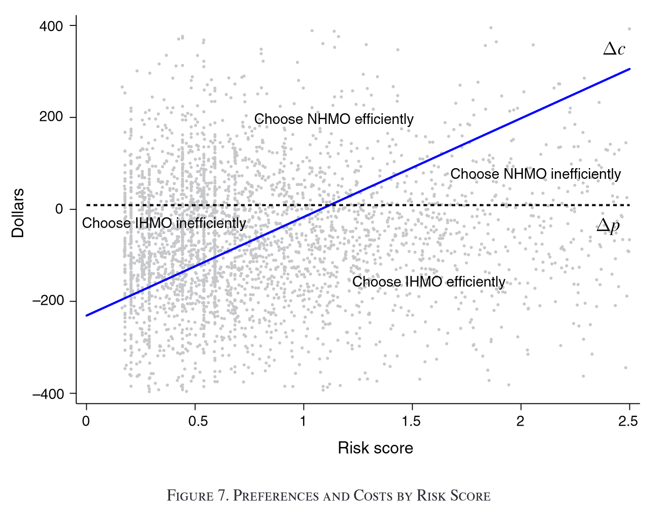
Takeaways
- Welfare loss of 2-11% of total cost of coverage under current pricing and contributions
- Uniform contribution policy (or community rating) offers modest improvements (1-3%)
- Risk-adjusted premium policy can capture entirety of welfare gains
References
Bundorf, M Kate, Jonathan Levin, and Neale Mahoney. 2012. “Pricing and Welfare in Health Plan Choice.” American Economic Review 102 (7): 3214–48.